Alternating Least Squares

Common steps for Recommendation Systems

import pandas as pd
import numpy as np

import matplotlib.pyplot as plt

ratings = pd.read_csv('/opt/datasetsRepo/RecommendationData/ratings.csv')
ratings.head()

	userId	movieId	rating	timestamp
0	1	1	4.0	964982703
1	1	3	4.0	964981247
2	1	6	4.0	964982224
3	1	47	5.0	964983815
4	1	50	5.0	964982931

idx_to_userid_mapper = dict(enumerate(ratings.userId.unique()))
userid_to_idx_mapper = dict(zip(idx_to_userid_mapper.values(), idx_to_userid_mapper.keys()))

idx_to_movieid_mapper = dict(enumerate(ratings.movieId.unique()))
movieid_to_idx_mapper = dict(zip(idx_to_movieid_mapper.values(), idx_to_movieid_mapper.keys()))

len(idx_to_userid_mapper), len(userid_to_idx_mapper)

(610, 610)

len(idx_to_movieid_mapper), len(movieid_to_idx_mapper)

(9724, 9724)

ratings['user_idx'] = ratings['userId'].map(userid_to_idx_mapper).apply(np.int32)
ratings['movie_idx'] = ratings['movieId'].map(movieid_to_idx_mapper).apply(np.int32)
ratings.head(10)

	userId	movieId	rating	timestamp	user_idx	movie_idx
0	1	1	4.0	964982703	0	0
1	1	3	4.0	964981247	0	1
2	1	6	4.0	964982224	0	2
3	1	47	5.0	964983815	0	3
4	1	50	5.0	964982931	0	4
5	1	70	3.0	964982400	0	5
6	1	101	5.0	964980868	0	6
7	1	110	4.0	964982176	0	7
8	1	151	5.0	964984041	0	8
9	1	157	5.0	964984100	0	9

References

• http://cs229.stanford.edu/proj2017/final-posters/5147271.pdf

• https://nightlies.apache.org/flink/flink-docs-release-1.2/dev/libs/ml/als.html

Intro

ALS algorithm works by alternating between rows and columns to factorized the matrix.

Stochastic Gradient Descent

• Flexibility - Already using it for a lot of different problems and algorithms

• Parallel - scaling matrix factorization

• Slower - iterative

• Hard to handle unobserved interaction (sparsity)

  Alternating Least Square

• only works for least square problems only

• Parallel

• Faster

• Easy to handle sparsity

Approach

            movies (n)                         k                  n
          +---------------------+        +------+   +----------------------+
          |                     |        |      | x |      movie           | k
          |                     |        | user |   |      factor          |      V
          |                     |        |factor|   +----------------------+
users(m)  |                     |        |      |
          |     RATINGS         |    ~   |      |
          |                     |    ~   |      | m
          |                     |        |      |
          |                     |        |      |
          |                     |        |      |
          +---------------------+        +------+
                                              U

Iterative Algorithm

• fix V, compute U

• fix U, compute V

Compare with SVD

Matrix Factorization Method.

More here https://machinelearningexploration.readthedocs.io/en/latest/MathExploration/SingularValueDecomposition.html

                                        +----------------------+
                                      K |______________________|
                                        |                      |
  items                            K    +----------------------+
+---------------------+        +-------+
|                     |        |   |   |
|u                    |        |   |   |
|s                    |        |   |   |
|e                    |    ~   |   |   |
|r                    |    ~   |   |   |
|s                    |        |   |   |
|                     |        |   |   |
|                     |        |   |   |
+---------------------+        +-------+
           X                      V       x       VT


                 row factors (items embeddings)
               /
Factorization
               \
                column factors (user embeddings)

In SVD the missing observations has to be fill as zeros.

\(| A - U V^T |^2\)

       item1  item2  item3   item4
      +------+------+------+------+
user1 |  1   |  0   |  0   |  1   |
      +------+------+------+------+
user2 |  0   |  1   |  0   |  0   |
      +------+------+------+------+
user3 |  0   |  1   |  0   |  0   |
      +------+------+------+------+
user4 |  0   |  0   |  1   |  0   |
      +------+------+------+------+

This leads to a large assumption for business and it impacts results heavily due to large percentage of assumptions.

In ALS we use rows and columns alternatively as features, hence no need to fill missing values.

\(\sum_{i,j \in obs} (A_{ij} - U_i V_j^T)^2\)

       item1  item2  item3   item4
      +------+------+------+------+
user1 |  1   |      |      |  1   |
      +------+------+------+------+
user2 |      |  1   |      |      |
      +------+------+------+------+
user3 |      |  1   |      |      |
      +------+------+------+------+
user4 |      |      |  1   |      |
      +------+------+------+------+

user_movie_matrix = ratings.pivot_table(values=['rating'] ,index=['user_idx'], columns=['movie_idx'])

user_movie_matrix.head(5)

	rating
movie_idx	0	1	2	3	4	5	6	7	8	9	...	9714	9715	9716	9717	9718	9719	9720	9721	9722	9723
user_idx
0	4.0	4.0	4.0	5.0	5.0	3.0	5.0	4.0	5.0	5.0	...	NaN	NaN	NaN	NaN	NaN	NaN	NaN	NaN	NaN	NaN
1	NaN	NaN	NaN	NaN	NaN	NaN	NaN	NaN	NaN	NaN	...	NaN	NaN	NaN	NaN	NaN	NaN	NaN	NaN	NaN	NaN
2	NaN	NaN	NaN	NaN	NaN	NaN	NaN	NaN	NaN	NaN	...	NaN	NaN	NaN	NaN	NaN	NaN	NaN	NaN	NaN	NaN
3	NaN	NaN	NaN	2.0	NaN	NaN	NaN	NaN	NaN	NaN	...	NaN	NaN	NaN	NaN	NaN	NaN	NaN	NaN	NaN	NaN
4	4.0	NaN	NaN	NaN	4.0	NaN	NaN	4.0	NaN	NaN	...	NaN	NaN	NaN	NaN	NaN	NaN	NaN	NaN	NaN	NaN

5 rows × 9724 columns

Algorithm

1. Initiate row factor U, column factor V

2. Repeat until convergence

   1. for i = 1 to n do (iterating over rows)

      \(u_i = (\sum_{r_{i,j} \in r_{i*}} {v_j v_j^T + \lambda I_k })^{-1} \sum_{r_{i,j} \in r_{i*}}{r_{ij} v_j}\)

   end for [solving for row factors when column factors are features]

   2. for i = 1 to m do (iterative over columns)

      \(v_i = (\sum_{r_{i,j} \in r_{*j}} {u_i u_i^T + \lambda I_k })^{-1} \sum_{r_{i,j} \in r_{*j}}{r_{ij} u_i}\)

   end for [solving for column factors when row factors are features]

Where

U = row factor matrix

V = column factor matrix

r = ratings

Similarity between als vs ols with l2 regularization

\(\theta = (X^T X + \lambda I)^{-1} X^T Y\)

\(v_i = (\sum_{r_{{i,j} \in r_{*j}}} {u_i u_i^T + \lambda I_k })^{-1} \sum_{r_{i,j} \in r_{*j}}{r_{ij} u_i}\)

Loss function

\begin{align*} R \approx U \times V^T\\ \\ \min_{U,V} \sum_{(i,j) \in \text{obs}} ( R_{i,j} - U_i V_j)^2 \end{align*}

def loss(R, U, V, M):
    # use by mask M to ignore NaNs
    return np.sqrt(np.square(R - (U @ V), where=M).sum())

Variables

factor dimensions, iteration, regularization

k = 2
n_iter = 20
lambda_ = 0.1

Rating Matrix

R = user_movie_matrix.values
n_users, n_movies = R.shape

Mask

M = ~np.isnan(R)

M

array([[ True,  True,  True, ..., False, False, False],
       [False, False, False, ..., False, False, False],
       [False, False, False, ..., False, False, False],
       ...,
       [ True,  True, False, ..., False, False, False],
       [ True, False, False, ..., False, False, False],
       [ True, False,  True, ...,  True,  True,  True]])

Factors initialization

u = np.random.rand(n_users, k)
v = np.random.rand(k, n_movies)

u.shape, v.shape

((610, 2), (2, 9724))

only getting observations (getting non null values from ratings)

obs = ~np.isnan(R[0])
v[:,obs] @ R[0,obs]

array([527.78422239, 515.52004112])

obs = ~np.isnan(R[:,0])
u[obs,:].T @ R[obs, 0], u.T[:,obs] @ R[obs, 0]

(array([422.3755339 , 419.93792029]), array([422.3755339 , 419.93792029]))

algorithm implemented

l_loss = []

for i_iter in range(n_iter):
    for i in range(n_users):
        # obs = ~np.isnan(R[i])
        obs = M[i] # same thing as above but already calculated and stored in a matrix
        u[i] = np.array((v[:,obs] @ R[i,obs]).T @ \
                        np.linalg.inv((v @ v.T) + (lambda_ * np.eye(k))))
    for j in range(n_movies):
        # obs = ~np.isnan(R[:,j])
        obs = M[:, j]
        v[:,j] = np.array((u.T[:, obs] @ R[obs,j]) \
                          @ np.linalg.inv((u.T @ u) + (lambda_ * np.eye(k))))
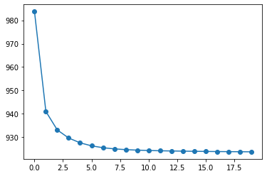
    l_loss.append(loss(R, u, v, M))

plt.plot(l_loss, 'o-');

in a function

def als(R, lambda_, dim_factors, n_iter):
    n_u, n_v = R.shape
    U = np.random.rand(n_u, dim_factors)
    V = np.random.rand(dim_factors, n_v)
    M = ~np.isnan(R)

    iter_losses = []
    for i_iter in range(n_iter):
        for i in range(n_u):
            obs = M[i]
            U[i] = np.array((V[:,obs] @ R[i,obs]).T @ \
                            np.linalg.inv((V @ V.T) + (lambda_ * np.eye(dim_factors))))
        for j in range(n_v):
            obs = M[:, j]
            V[:,j] = np.array((U.T[:, obs] @ R[obs,j]) @ \
                              np.linalg.inv((U.T @ U) + (lambda_ * np.eye(dim_factors))))
        iter_losses.append(loss(R, U, V, M))
    return U,V,iter_losses

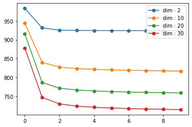
comparing incremental factor dimensions

dims = [2, 10, 20, 30]
for dim in dims:
    _, _, losses = als(R, 0.1, dim, 10)
    plt.plot(losses, 'o-', label=f"dim : {dim}")

plt.legend(loc='best')
plt.show()

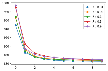
comparing incremental regularization rate

lambdas_ = [0.01, 0.09, 0.1, 0.5, 0.9]
for reg in lambdas_:
    _, _, losses = als(R, reg, 5, 10)
    plt.plot(losses, 'o-', label=f"$\lambda$ : {reg}")

plt.legend(loc='best')
plt.show()

Weighted Alternating Least Squares (WALS)

\begin{align} \sum_{i,j \in obs} (A_{ij} - U_i V_j)^2 + w_k \times \sum_{i,j \notin obs} (0 - U_i V_j)^2 \end{align}